RP 48 – Low-Cost Threat Intelligence & Honeypot Project

Full documentation: ML training, datasets, hyperparameters, accuracy, honeypot operation, project run, simulation, model artifacts (PKL/JSON), and dashboard screenshots.

1. Project Deliverables (Scope)

1.1 Hybrid honeypot deployment

The project deploys an advanced hybrid honeypot: one process provides real SSH (via Paramiko) on port 2222 and Telnet on port 2323. SSH supports full key exchange and password auth, a persistent host key (data/honeypot_keys/), an interactive shell with a virtual filesystem (ls, cd, cat, pwd, whoami, id, uname, etc.), and single-command exec (e.g. ssh user@host "cat /etc/passwd"). Telnet presents an Ubuntu-style login prompt and captures credentials. Every connection is logged as soon as it is accepted; a queue-based writer thread ensures logs are not dropped under high load (e.g. DDoS). All events go to data/honeypot_logs.jsonl. The implementation is split into multiple modules (config, filesystem, logger, SSH/Telnet handlers) for maintainability.

1.2 MITRE ATT&CK mapping

Every honeypot event is mapped to one or more MITRE ATT&CK technique IDs. The mapping is implemented in attack_mapping/mitre_map.py and attack_mapping/map_events.py. Examples: login_attempt / brute_force → T1110.001 (Password Guessing); connection / raw_input → T1595.002; command → T1059.004, T1021.001; DDoS → T1498. The export script applies this mapping so the dashboard and any downstream dataset use technique IDs.

1.3 Threat intelligence dashboard

A React dashboard in dashboard/ provides the threat intelligence UI. It loads event data from dashboard/public/events.json (generated by scripts/export_events_for_dashboard.py from honeypot logs). The dashboard shows: Overview (KPIs, honeypot attacks bar, attacks histogram, attack map, time series by service/event type, donuts), Threat Events table, Geo Map, Analytics (events over time, by service), Top IPs, and ATT&CK Matrix (technique badges). All views use real data only (no mock data).

1.4 Reusable dataset

The reusable dataset consists of (1) cleaned IDS data in data/ (e.g. unsw_nb15_cleaned.parquet, cic_ids2018_cleaned.parquet) produced by the data-cleaning notebook, and (2) honeypot-derived events with ATT&CK technique IDs. The latter is the same data as events.json; the source log is data/honeypot_logs.jsonl. Exported events can be used for research, ML, or sharing TTPs.

1.5 Validation

Validation is done in two ways: (1) ML validation and test metrics from ml/train.py (accuracy, precision, recall, F1 on a held-out test set; validation vs test bar chart saved under models/). (2) Honeypot/attack simulation: run python scripts/simulate_ddos_honeypot.py against localhost to generate many connections; then run the export script and refresh the dashboard to confirm events and ATT&CK mapping appear correctly.

2. ML Training

2.1 How training works

Training is implemented in ml/train.py. The script:

1. Loads a dataset (raw from datasets/ or cleaned from data/).
2. Prepares features X and labels y (multi-class from attack_cat or Label; binary from label if used).
3. Splits into train (64%), validation (16%), and test (20%) with stratification.
4. Optionally adds label noise to training labels when HARDER_MODE=1 (see Special codes).
5. Fits StandardScaler on training data and scales train/val/test.
6. Trains XGBoost for 100 rounds with a custom callback to record validation accuracy, precision, recall, F1 per iteration.
7. Trains LOF on scaled training data for anomaly detection.
8. Saves model, scaler, LOF, feature names, class names, and plots under models/.

2.2 Datasets used

Priority order:

If the combined UNSW data has more than 200,000 rows, a stratified sample of 200,000 is used for training.

2.3 Hyperparameters

2.4 Accuracy and metrics

After training, the script prints validation and test metrics (accuracy, precision, recall, F1). Test metrics are computed on the held-out 20% and are the main measure of performance. Reported results (UNSW-NB15 raw, Train: 128000, Val: 32000, Test: 40000):

XGBoost Test Results (Held-out):
  Accuracy:  0.8057
  Precision: 0.6887
  Recall:    0.4481
  F1 Score:  0.4547

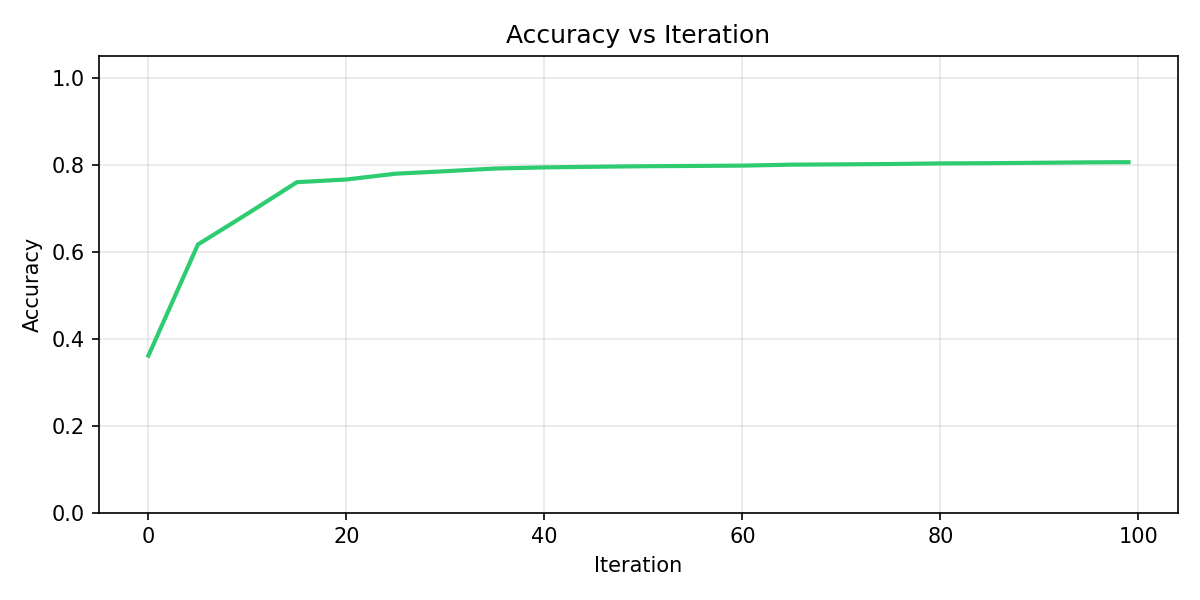
Validation metrics over iterations are stored in models/training_history.json. During training the script also saves the following graphs to models/; copies are included in doc/ for documentation.

2.4.1 Accuracy vs iteration

This graph plots validation accuracy (y-axis) against iteration (x-axis, 0–100). Accuracy starts low (around 0.35), rises quickly in the first ~20 iterations (to about 0.77–0.80), then stabilizes. The plateau indicates the model has converged; extra iterations beyond ~40 give little gain. It shows how many rounds are needed for stable performance and helps decide whether to reduce or increase num_boost_round.

2.4.2 Confusion matrix (test set)

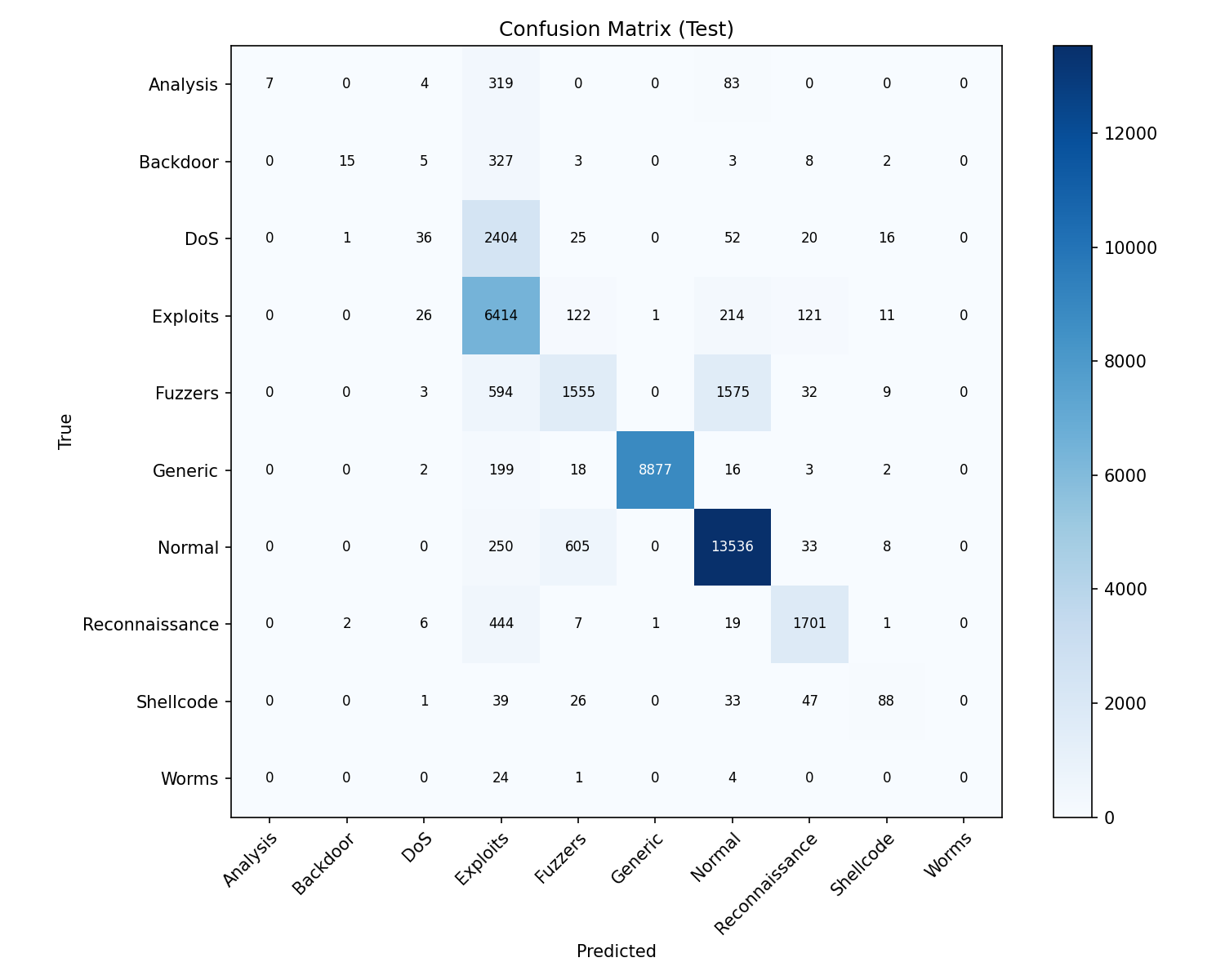
The confusion matrix compares true labels (y-axis) with predicted labels (x-axis) on the held-out test set. Each cell (i, j) is the count of samples that are truly class i but predicted as class j. The diagonal (true class = predicted class) are correct predictions; off-diagonal cells are errors. Darker blue means higher count. From this we see: Generic and Normal have many correct predictions; Exploits are well detected; Analysis, Backdoor, DoS, and Worms are often missed or confused with Exploits; Fuzzers are sometimes confused with Normal. This pinpoints which classes need more data or feature work.

2.4.3 Per-class metrics (test set)

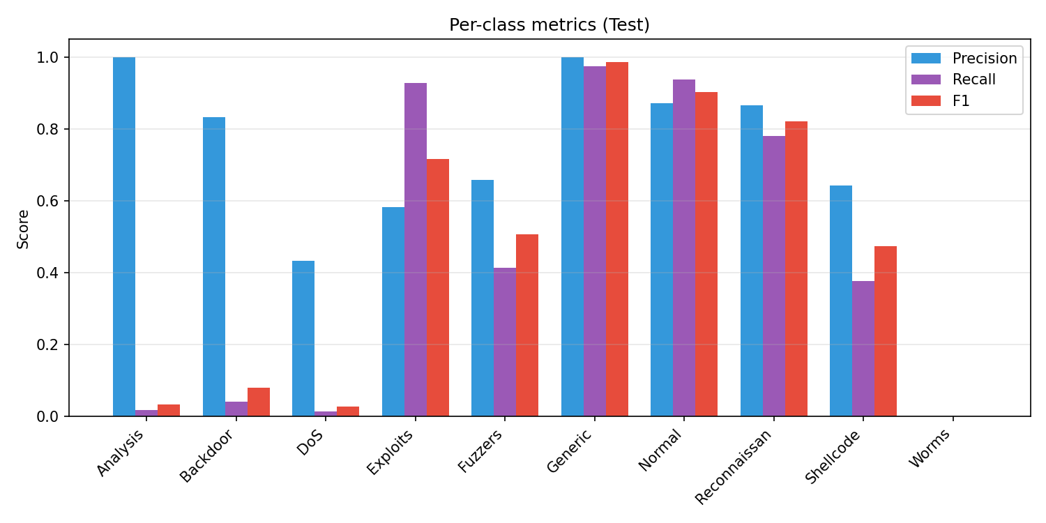
This bar chart shows Precision (blue), Recall (purple), and F1 score (red) for each attack class on the test set. Generic and Normal have high scores across all three; Exploits and Reconnaissance are solid. Analysis, Backdoor, DoS, and Worms have very low recall (the model misses most of these), and Worms has zero precision/recall/F1. High precision with low recall (e.g. Analysis, Backdoor) means the model is right when it predicts that class but rarely predicts it. This graph complements the confusion matrix by summarizing per-class performance in one view.

2.5 Models used and why

• XGBoost: Used for attack vs normal (or multi-class attack type). It handles mixed feature types, is fast with tree_method='hist', and supports strong regularization to reduce overfitting. Performs well on tabular IDS data.
• Local Outlier Factor (LOF): Used for unsupervised anomaly detection. It flags samples with low local density (outliers). Complements the classifier by highlighting flows that do not resemble the training distribution. Trained on scaled features; n_neighbors=20, contamination=0.05.

3. Model Artifacts (PKL and JSON files)

All artifacts are saved under models/.

Inference: ml/predict.py loads these artifacts via load_artifacts(), then predict(X) returns label, anomaly, and optionally class (class names for multi-class).

4. Honeypot: How It Works

4.1 Architecture (multiple files)

The honeypot is split into modules under honeypot/:

4.2 SSH (port 2222)

• Real SSH protocol via Paramiko: key exchange, password authentication (any password accepted), session and PTY.
• Persistent host key: stored in data/honeypot_keys/ssh_host_rsa_key; generated once, reused so clients can accept the key once.
• Interactive shell: prompt root@server:/root#; supports ls, cd, pwd, cat, head, tail, whoami, id, uname (-a/-r), wget/curl (simulated “connection refused”), help, exit. Other commands return “command not found”.
• Exec channel: single-command execution (e.g. ssh root@host "cat /etc/passwd") is supported; command and output are handled via the same virtual filesystem.
• Events logged: connection (at accept), login_attempt (username/password), command (each shell or exec command).

Test from a second terminal: ssh -o StrictHostKeyChecking=accept-new -p 2222 root@localhost (any password).

4.3 Telnet (port 2323)

• Presents an Ubuntu-style banner and server login: / Password: prompts.
• Captures username and password, logs login_attempt, then responds with “Login incorrect”.
• connection is logged at accept time (same as SSH).

4.4 Logging and DDoS resilience

• Each new TCP connection is logged with event_type: connection and service (ssh/telnet) as soon as it is accepted, before the handler runs. Under connection floods, every connection is still recorded.
• log_event() pushes a JSON object to an in-memory queue; a single writer thread appends one line per event to data/honeypot_logs.jsonl. This avoids many threads writing to the same file and reduces the risk of dropped or corrupted logs under load.
• Log fields: timestamp, source_ip, service, event_type, and optionally username, password, command, raw.

5. How to Run the Project

1. Environment: python -m venv venv, venv\Scripts\activate, pip install -r requirements.txt. For the dashboard: cd dashboard && npm install.
2. Data (optional for ML): Place raw UNSW-NB15 or CIC-IDS2018 in datasets/. Alternatively run notebooks/data_cleaning.ipynb to produce cleaned data in data/.
3. Train ML: python ml/train.py. Outputs and plots go to models/.
4. Honeypot: python honeypot/server.py. Leave running; logs go to data/honeypot_logs.jsonl. In a second terminal, test SSH: ssh -o StrictHostKeyChecking=accept-new -p 2222 root@localhost (any password).
5. Export for dashboard: python scripts/export_events_for_dashboard.py. Writes dashboard/public/events.json with ATT&CK-mapped events.
6. Dashboard: cd dashboard && npx vite (or npm run dev). Open the URL shown (e.g. http://localhost:5173). The dashboard fetches /events.json and shows real data only.

6. Simulating Honeypot Attack (Load Test)

To generate many connections against your own honeypot (localhost only):

python scripts/simulate_ddos_honeypot.py

Options:

• -n 200: number of connection attempts (default 100).
• -t 20: number of concurrent threads (default 20).
• --port 2323: target Telnet instead of SSH (2222).
• --login: send root\n so some events are logged as login_attempt.

Example:

python scripts/simulate_ddos_honeypot.py -n 500 -t 50 --login

Then run python scripts/export_events_for_dashboard.py and refresh the dashboard to see the new events. The script only allows 127.0.0.1 or localhost as the target host.

To add sample log lines (e.g. for demo) without running the honeypot: python scripts/add_sample_logs.py. Then export and refresh the dashboard as above.

7. Special Codes and References

8. Data Cleaning Notebook

notebooks/data_cleaning.ipynb cleans the raw UNSW-NB15 and CSE-CIC-IDS2018 datasets for use in the ML pipeline.

• UNSW-NB15: Loads UNSW_NB15_training-set.csv and UNSW_NB15_testing-set.csv from datasets/UNSW-NB15/. Explores dtypes, labels, and attack categories. Fills numeric NaNs with column medians (in a single assignment to avoid chained assignment). Writes data/unsw_nb15_cleaned.parquet and data/unsw_nb15_cleaned.csv.
• CSE-CIC-IDS2018: Loads CIC data from datasets/CSE-CIC-IDS2018/ (e.g. cic.csv). Cleans and normalizes columns, handles labels. Writes data/cic_ids2018_cleaned.parquet and data/cic_ids2018_cleaned.csv.

The ML script can use either the raw datasets in datasets/ or these cleaned outputs in data/ (raw is preferred when available to avoid any cleaning-induced bias).

9. Dashboard Screenshots (doc/)

Place screenshots of the dashboard in the doc/ folder. Below is what each main view shows and how it relates to the project.

9.1 Overview

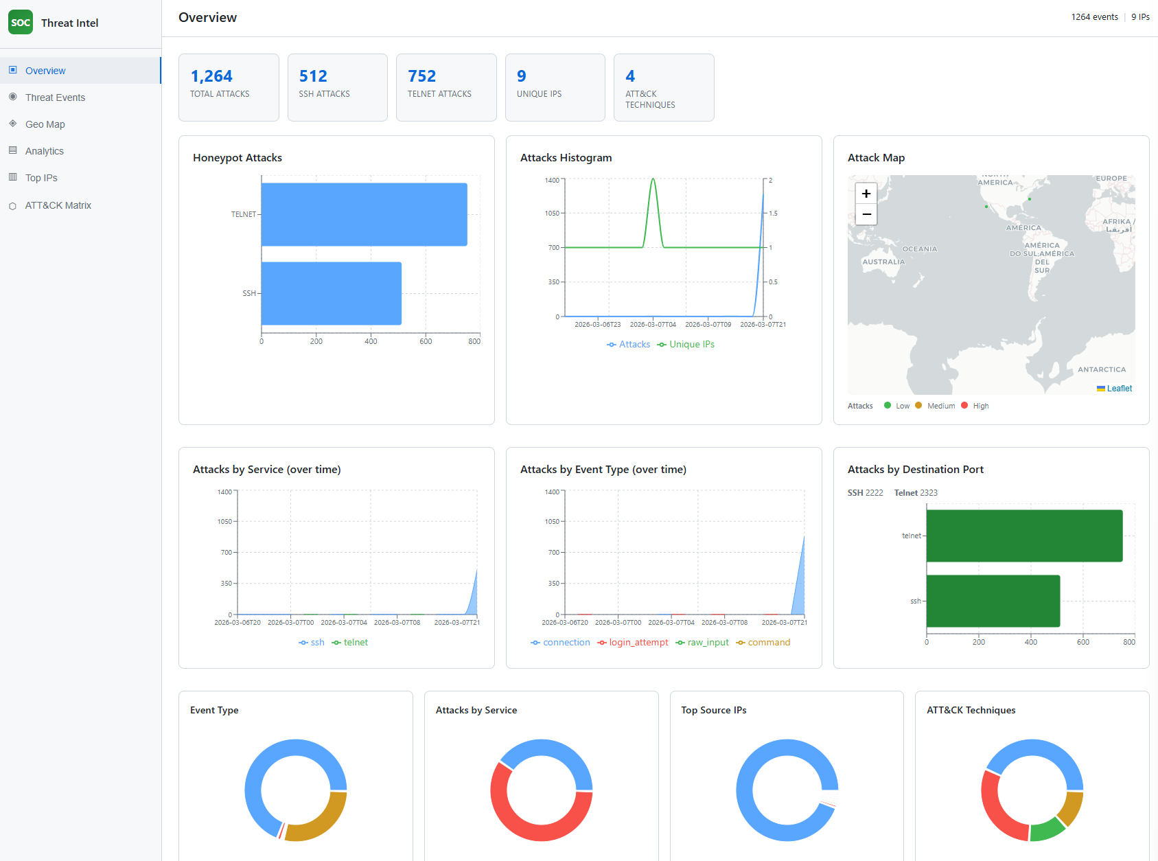
Screenshot: doc/Screenshot 2026-03-08 033031.png (Overview).

The Overview tab shows the SOC Threat Intel dashboard home: summary KPI cards (Total Attacks, SSH Attacks, Telnet Attacks, Unique IPs, ATT&CK Techniques), a bar chart of honeypot attacks by service (SSH vs Telnet), an attacks histogram (attacks and unique IPs over time), an attack map with a Low/Medium/High legend, time series of attacks by service and by event type, a bar chart of attacks by destination port (SSH 2222, Telnet 2323), and four donut charts (Event Type, Attacks by Service, Top Source IPs, ATT&CK Techniques). This view demonstrates the threat intelligence dashboard and the hybrid honeypot deployment (two services, two ports) and how ATT&CK technique counts are surfaced.

9.2 Threat Events

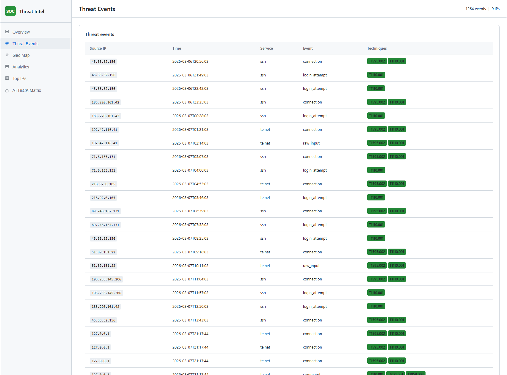
Screenshot: doc/Screenshot 2026-03-08 033041.png (Threat Events).

The Threat Events tab shows a table of individual events: Source IP, Time, Service, Event type, and Techniques (MITRE ATT&CK IDs as badges). This illustrates how each honeypot event is mapped to techniques (MITRE ATT&CK mapping) and how the reusable dataset is structured (each row is an event with technique IDs).

9.3 Geo Map

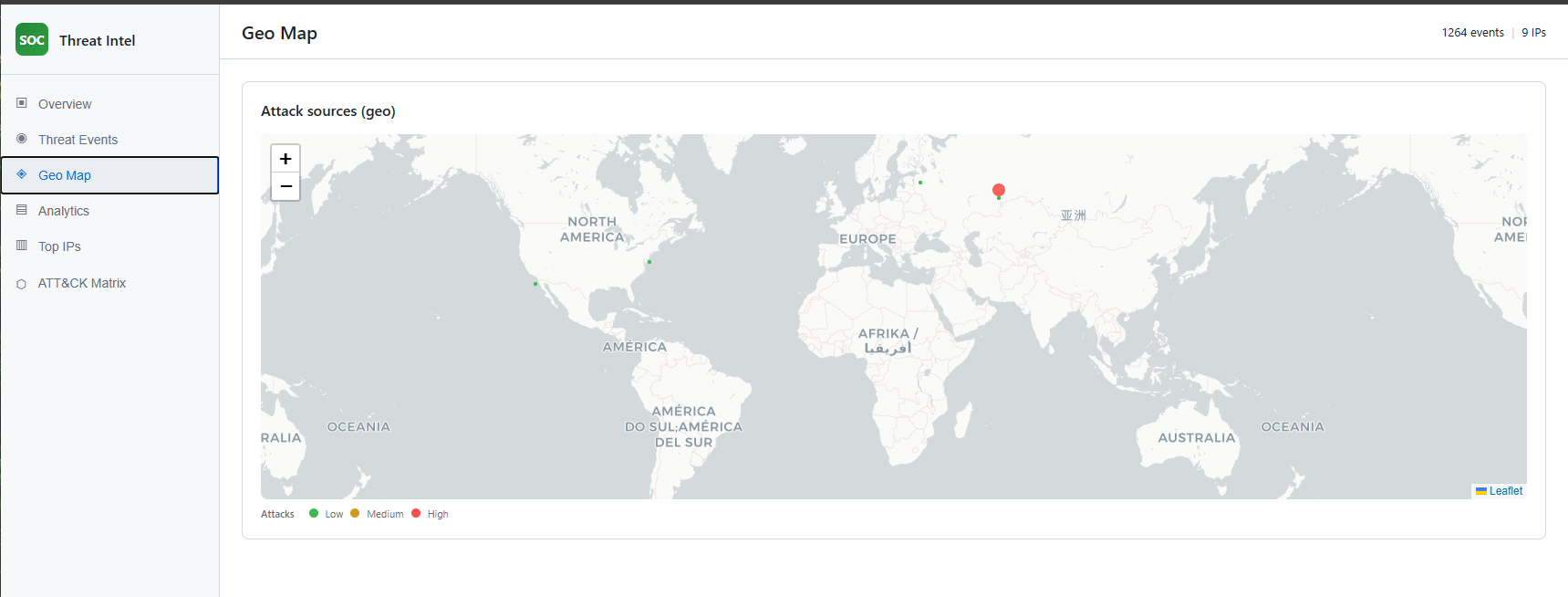
Screenshot: doc/Screenshot 2026-03-08 033118.png (Geo Map).

The Geo Map tab shows a world map with markers for attack sources. Marker size and color indicate intensity (Low / Medium / High). The map uses a light basemap and places IPs into regions (e.g. Russia, US, Sri Lanka) for visualization. This supports the threat intelligence dashboard by providing geographical context for the honeypot data.

9.4 Analytics

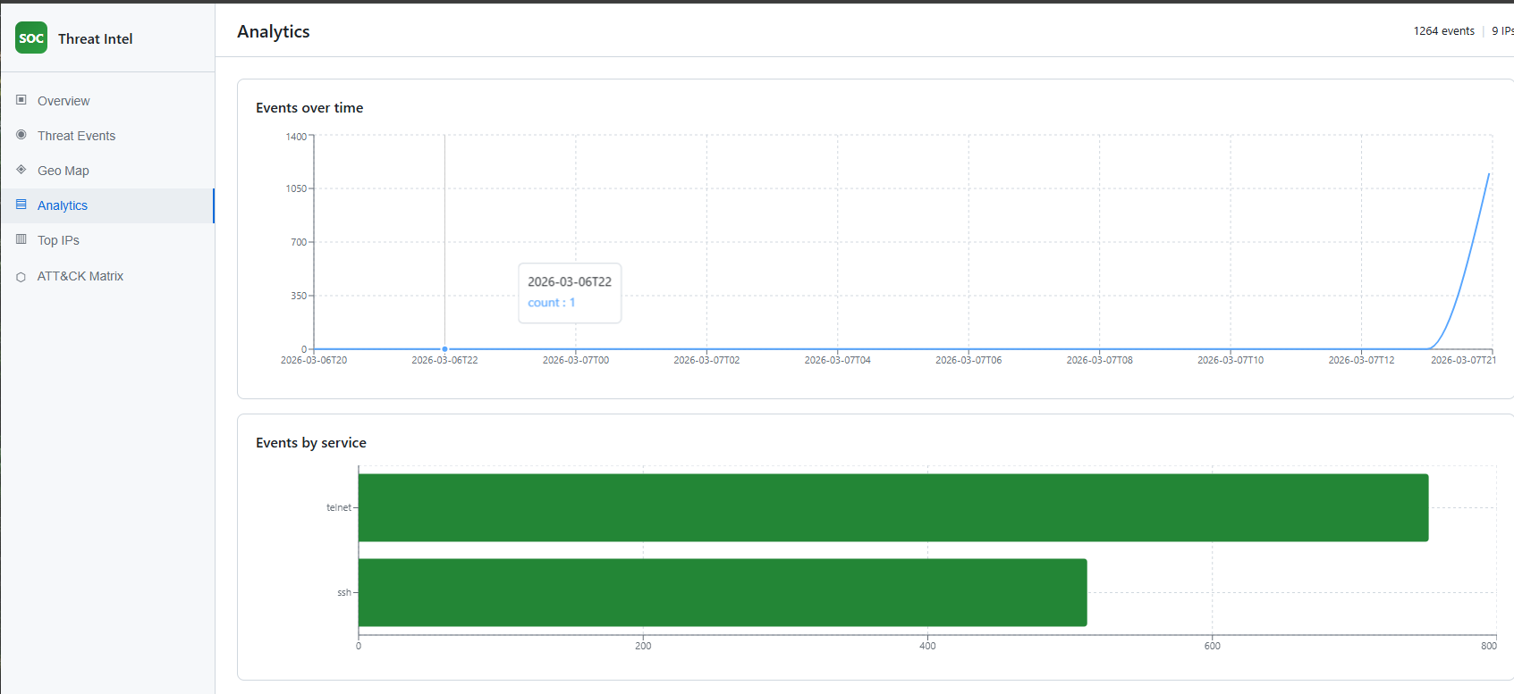
Screenshot: doc/Screenshot 2026-03-08 033048.png (Analytics).

The Analytics tab shows “Events over time” (line chart of event count per hour) and “Events by service” (horizontal bar chart for SSH and Telnet). This demonstrates how the dashboard visualizes trends and service mix from the honeypot, and supports validation by showing that simulated or real traffic appears in the expected time windows and services.

9.5 Top IPs

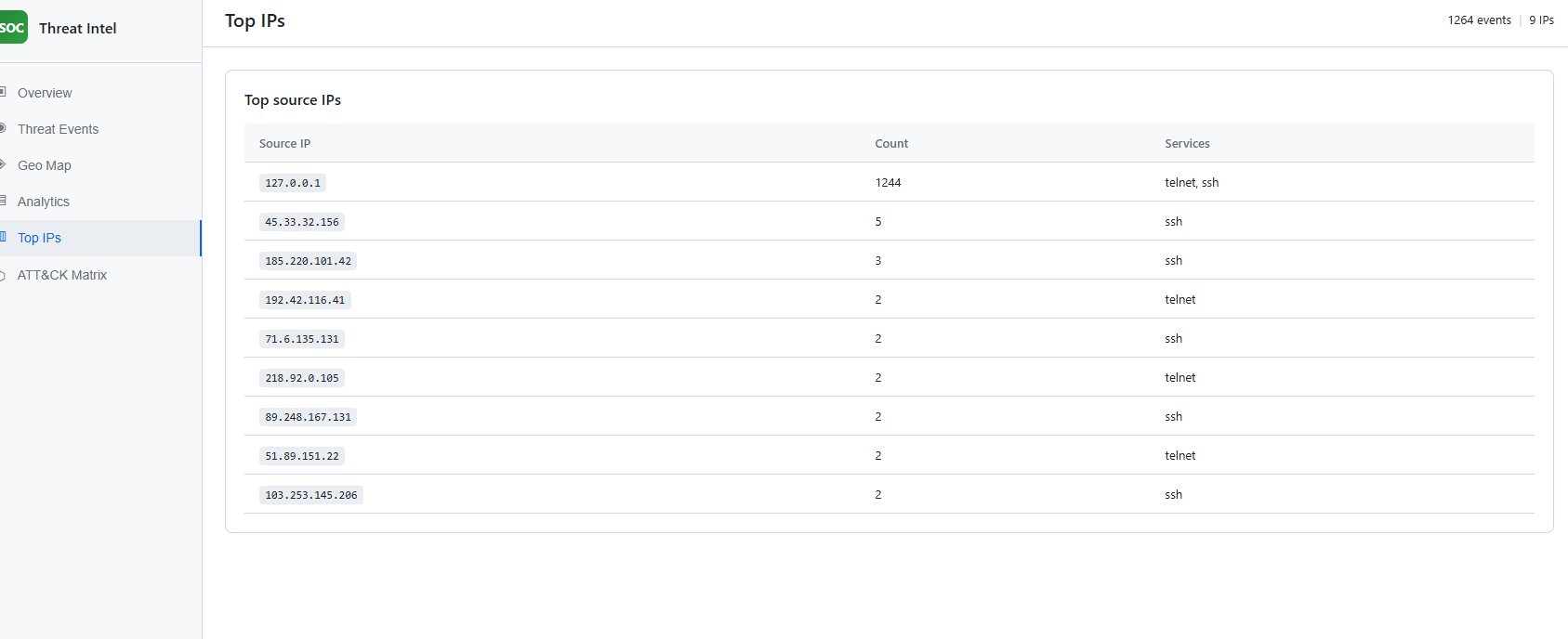
Screenshot: doc/Screenshot 2026-03-08 033130.png (Top IPs).

The Top IPs tab lists the most active source IPs with event count and services (e.g. ssh, telnet). It helps identify which IPs are generating the most traffic to the honeypot. Localhost (127.0.0.1) with a high count typically indicates local simulation runs.

9.6 ATT&CK Matrix

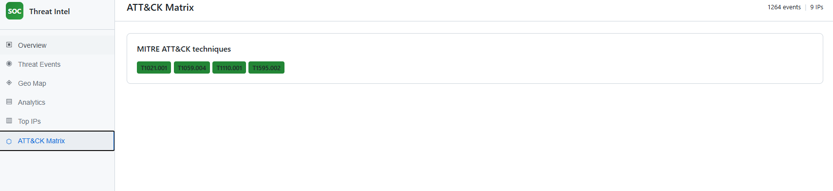
Screenshot: doc/Screenshot 2026-03-08 033133.png (ATT&CK Matrix).

The ATT&CK Matrix tab shows the list of observed MITRE ATT&CK technique IDs (e.g. T1021.001, T1059.004, T1110.001, T1595.002) as badges. This is the direct view of MITRE ATT&CK mapping output: which techniques were inferred from the honeypot events.

10. Summary

• Advanced hybrid honeypot: Multi-file implementation under honeypot/ (config, filesystem, logger, ssh_handler, telnet_handler, server). Real SSH (Paramiko) on 2222 with persistent host key, interactive shell and virtual filesystem, exec support; Telnet on 2323 with login prompt. Connection logged at accept; queue-based logging for DDoS resilience; logs to data/honeypot_logs.jsonl.
• MITRE ATT&CK mapping: attack_mapping/mitre_map.py and map_events.py; export script adds mitre_techniques to events for the dashboard and dataset.
• Threat intelligence dashboard: React app in dashboard/; loads events.json; shows Overview, Threat Events, Geo Map, Analytics, Top IPs, ATT&CK Matrix.
• Reusable dataset: Cleaned IDS data in data/; honeypot events with ATT&CK IDs in events.json and source log honeypot_logs.jsonl.
• Validation: ML test metrics from ml/train.py; honeypot validation via scripts/simulate_ddos_honeypot.py and dashboard verification.